GROMACS 4.6 example: n-phenylglycinonitrile binding to T4 lysozyme

Free Energy Fundamentals
Theory Definitions Exponential Averaging / Zwanzig Thermodynamic Integration Bennett Acceptance Ratio WHAM MBAR
Methods of Free Energy Simulations Thermodynamic Cycle Intermediate States (Constructing) Soft Core Potentials Running Simulations Extracting Simulation Information Analysis / Bootstrap Sampling
Improving Sampling and Accelerating Simulations Umbrella Sampling Hamiltonian Replica Exchange [math]\displaystyle{ \lambda }[/math]-dynamics / Expanded Ensemble

Free Energy How-to's
Example Calculations Absolute Solvation Free Energy Relative Binding Affinity Absolute Binding Affinity
Tutorials Ethanol Solvation - GROMACS Expanded Ensemble - GROMACS Absolute Binding Free Energy - GROMACS

Introduction

In this tutorial we will try to obtain the free energy of binding of n-phenylglycinonitrile to T4 lysozyme using an alchemical pathway, in order to reproduce the result obtained in the published work of Boyce et al. 2009. In particular, we will start from the holo structure (PDB code 2RBN).

The tutorial assumes knowledge of Gromacs 4.6 and basics of free energy calculations. Before this practical, I would also suggest going through >this< ethanol solvation tutorial on alchemistry.org, or >this< methane solvation tutorial written by Justin Lemkul.

The thermodynamic cycle used to obtain the results will be reviewed first, and then we will go through the principal steps of the process. The input files needed to run the calculations will be provided, however you can also set everything up from scratch by yourself if you wish (it can be a good exercise in fact).

For enquiries about the tutorial please feel free to email me.

Thermodynamic cycle

Here is a graphical representation of the cycle we will use in this tutorial, as I find it helpful to visualise the steps needed to carry out the calculations. It's purpose is simply to summarise the steps we will need to consider - if this seems confusing, I would suggest visiting the following pages before proceeding with the tutorial: thermodynamic cycle, absolute binding affinty.

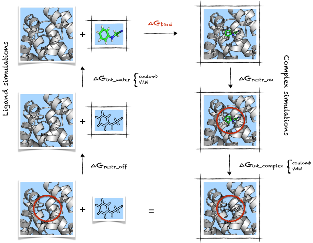
In the cycle above, the systems we need to simulate are indicated by having a black box around them, restraints are indicated by a red circle, the transparent ligand means it is not interacting with the environment and the light blue background is reminding that water is present. The right column has the simulations involving the complex, whereas the left column the simulations involving only the ligand.

Starting from the top-right corner we have the complex, with the ligand (n-phenylglycinonitrile) and protein (T4 lysozyme) fully interacting as in a normal MD simulation. Now we want to decouple the ligand from the system in order to get to the bottom-right corner of the cycle. This will involve running a number of separate simulations at different lambda values, first decoupling coulombic interactions and then Lennard-Jones ([math]\displaystyle{ \Delta G_{int\_complex} }[/math]).

However, before doing this we will need to add a set of restraints between ligand and protein (giving [math]\displaystyle{ \Delta G_{restr\_on} }[/math]) in order to avoid the problem of the ligand leaving the binding pocket when interactions are being removed. The presence of restraints is indicated in the cycle scheme above by a red circle, which is trying to represent the fact that the ligand is being confined to a certain volume. The set of restraints described by Boresch is used for this work. These are quite useful as they restrain position and orientation of the compound relative to the protein, and they have an analytical solution for their removal that also includes a correction for the standard state.

Going up from the bottom-left corner of the cycles, the first step ([math]\displaystyle{ \Delta G_{restr\_off} }[/math]) will then be carried out analytically without need to run more simulations. At this point we want the ligand to come back to interact with the solvent, which means we need to turn on charges and Van der Waals parameters again, in order to obtain [math]\displaystyle{ \Delta G_{int\_water} }[/math]. In practice we will be doing the opposite, that is decoupling the ligand from the water box; however, note how this means running basically the same set of simulations. This also results in the same free energy difference, just with opposite sign.

At this point we are finally at the top-left corner of the cycle, which means that summing up all the steps done so far we are going to obtain the quantity we are after: [math]\displaystyle{ \Delta G_{bind} }[/math]. Or, in fact, its opposite since we went from bound to unbound state.

Initial setup

In order to have everything ready to run the windows at different lambda values we need to have the input files ready (.gro, .top and .mdp files); the typical GROMACS editconf/genbox/genion steps apply. Briefly, for this exercise the setup is as follows: dodecahedral box with minimum distance of 1.0 nm from the protein, Amber99SB-ILDN force field, TIP3P water model, GAFF parametrization for the ligand with AM1-BCC charges. More details about the parameters are in the .mdp files provided.

You can find the input files needed to complete the tutorial here: Input Files. Note that in the .mdp files, init-lambda-state is not defined (it has a meaningless 'X' value at the moment), as you will need to create as many .mdp files as the number of lambda states present. This is explained also later on in the text.

Complex

For consistence with the description of the cycle above, we will start taking care of the simulations involving the complex. This set of simulations involve a total of 30 windows, and for each of them energy minimization, NVT and NPT equilibration, and production run (1 ns) have to be performed.

It is worth briefly discussing some points about the topology file:

• Note how the protein and ligand have been joined in a single [ moleculetype ]. This is at the moment (GROMACS 4.6.x) necessary in order to apply restraints between ligand and protein (although it seems there is some work in progress about this...have a look at this discussion on the GROMACS forum if you want to know more: here). It follows that in this way it is necessary to merge the two topologies by changing the atoms indices for the ligand.

• States A and B for the system are defined. In state B, all ligand atoms have zero charge and a different atom type. The new "dummy" atom types are defined under the [ atomtypes ] section and are given zero Van der Waals parameters. However, since we would like to decouple the ligand rather than annihilate it, the [ nonbonded_params ] section is defined and it overrides the mixing rules for LJ parameters. Note that the charges are instead simply annihilated, as it is currently not possible to retain the intramolecular coulombic interactions when setting up the calculations by topology modification.

• The set of restraints we use comprises 1 distance, 2 angles and 3 dihedrals. Angles and dihedrals restraints are defined in the topology, whereas the distance restraint is here applied through the pull code and it is therefore defined in the .mdp files. Also, the index.ndx file is then needed to define the two groups (atoms) used by the pull code.

In the .mdp files we then define 3 lambda vectors: restraints, coulomb and vdw. This way we can use 30 identical .mdp files where we simply choose the state we are simulating with init-lambda-state. As it is possible to see, we first apply the restraints, then we remove the coulombic and finally the Van der Waals interactions.

We are now ready to run all the simulations and collect all the dhdl.xvg files needed for analysis. Then we can analyse the results with the alchemical-gromacs.py scripts provided with pyMBAR:

   python alchemical-gromacs.py -d 'directory' -p 'prefix' -t 300 -s 100 -u kcal -v

To see the help for the script just run it with the '-h' flag, so that it will show the meaning of all the options too. If you prefer, you can also use GROMACS' g_bar; however I find pyMBAR and alchemical-gromacs.py much more convenient as it already subsamples the data after calculating the statistical inefficiency, estimates the free energy with various methods (including BAR, MBAR and TI) and prints out results and some useful plots in a tidy format.

For this step, with MBAR I obtained:

[math]\displaystyle{ \Delta G_{restr\_on} + \Delta G_{int\_complex} = 23.797 \pm 0.050 \ kcal/mol }[/math]

Here a link to a summary of the results: Results for complex. Note that this might not be exactly the number you will get (even if you use exactly the same input files, parameters and GROMACS version I used) but it gives an idea of what sort of value one should expect. In fact, running two additional complex calculations, I obtained a standard deviation for the three runs of 0.69 kcal/mol.

Removal of Restraints

Now the ligand is decoupled from the protein (and the solvent). The next step in the cycle is to remove the restraints. As mentioned before, with this choice of restraints we can derive the free energy of restraints removal analytically. The formula to use is the following, but I would suggest to first read the relevant paper to understand what it means.

[math]\displaystyle{ \displaystyle \Delta G_{restr\_off} = -kT \ln\Bigg[ \frac{8 \pi^{2}V^{0}}{r_{0}^{2} sin \theta_{A,0} sin \theta_{B,0}} \frac{(K_r K_{\theta_{A}} K_{\theta_{B}} K_{\phi_{A}} K_{\phi_{B}} K_{\phi_{C}})^{\frac{1}{2}}}{(2 \pi k T)^{3}}\Bigg] }[/math]

Where:

[math]\displaystyle{ k }[/math] is the ideal gas constant;

[math]\displaystyle{ T }[/math] is the temperature in Kelvin;

[math]\displaystyle{ V^{0} }[/math] is the volume corresponding to the one molar standard state (1660 [math]\displaystyle{ \AA^3 }[/math]);

[math]\displaystyle{ r_0 }[/math] is the reference distance for the restraints;

[math]\displaystyle{ \theta_{A}, \theta_{B} }[/math] are the reference angles for the restraints;

[math]\displaystyle{ K_x }[/math] is the force constant for the distance ([math]\displaystyle{ r_0 }[/math]), two angles ([math]\displaystyle{ \theta_{A}, \theta_{B} }[/math]) and three dihedrals ([math]\displaystyle{ \phi_{A}, \phi_{B}, \phi_{C} }[/math]) restraints we applied.

If you are using exactly the set of restraints provided with the input files, this should give:

[math]\displaystyle{ \Delta G_{restr\_off} = -6.906 \ kcal/mol }[/math].

Ligand in Water

The same considerations discussed for the complex simulations apply for the ligand as well. State B has zero charges and dummy atom types and we need to run 20 simulations of the ligand in water, at the different states defined by the lambda vectors in the .mpd files. In this case we are only turning off coulombic and Lennard-Jones interactions, since the restraints have just been accounted for analytically.

The results can be obtained again in the same way as we did for the complex. Here a link to what I obtained after running alchemical-gromacs.py: (Results for ligand). MBAR gives me:

[math]\displaystyle{ \Delta G_{int\_water} = 11.412 \pm 0.017 \ kcal/mol }[/math]

Long Range Dispersion Correction

At this point we have carried out all the simulations we need to reproduce the result obtained by Boyce 2009. However, the authors also applied a long range dispersion correction to their final results. The EXP-LR method is described in Shirts et al., J. Phys. Chem. B, 2007. What it does is basically correcting for the fact we are using a cutoff for the Van der Waals term in a nonisotropic system. Again, the best thing to do to have an idea of why and how this is done is probably to read the original paper.

In order to obtain the correction, we need to rerun the first (fully interacting, [math]\displaystyle{ \lambda = 0 }[/math]) and last (non-interacting, [math]\displaystyle{ \lambda = 1 }[/math]) lambda states of the Van der Waals transformation (i.e. init-lambda-state 14 and 29 in our case) for the complex, using the largest cut-offs we can for the box size we have (which should be around 3.8 nm). This can be done using the -rerun flag for mdrun and providing the trajectory file, for example:

   mdrun -rerun prod.14.xtc -s long.14.tpr -deffnm long.14 -v

Where long.14.tpr is the new .tpr file that we created modifying the .mdp file for lambda state 14 in order to have a large rvdw cutoff.

Since we are reprocessing with a long cut-off only the (infrequently) stored configurations, and we would like to compare the same configurations with long and short cutoffs, we can rerun the two lambda states also with the original .mdp file with a short vdw cutoff. g_energy can give us a free energy estimate using exponential averaging; so we can use it to compute the free energy of extending the cutoff for the end states ([math]\displaystyle{ \lambda = 0 }[/math] and [math]\displaystyle{ \lambda = 1 }[/math]) of the VdW transformation:

   g_energy -f short.14.edr -f2 long.14.edr -fee -o exp-lr.14 -fetemp 300

   g_energy -f short.29.edr -f2 long.29.edr -fee -o exp-lr.29 -fetemp 300

In this way I obtained [math]\displaystyle{ \Delta G^{LR}(\lambda = 1) = -17.594 \ kcal/mol }[/math] and [math]\displaystyle{ \Delta G^{LR}(\lambda = 0) = -18.283 \ kcal/mol }[/math], which results in a correction of:

[math]\displaystyle{ \Delta G^{LRC} = 0.688 kcal/mol }[/math]

This value will be added to the free energy computed for the complex and will contribute to a higher affinity.

Final Results

Now it's time to pull everything together. In summary:

[math]\displaystyle{ \Delta G_{complex} = \Delta G_{restr\_on} + \Delta G_{int\_complex} + \Delta G^{LRC} = 24.485 \ kcal/mol }[/math]

[math]\displaystyle{ \Delta G_{int\_water} = -11.412 \ kcal/mol }[/math] (with this sign because we 'desolvated' the ligand, but in the cycle we need to 'solvate' it)

[math]\displaystyle{ \Delta G_{restr\_off} = -6.906 \ kcal/mol }[/math]

Summing everything we obtain the free energy of dissociation, so if we want the free energy of binding we simply take the negative of it. This, in my case, results in:

[math]\displaystyle{ \Delta G_{bind} = -6.17 \ kcal/mol }[/math]

The published result is -6.09 kcal/mol, which is quite close in this instance. However, it is possible you'll get something slightly different. In fact, considering the final free energies I would obtain if I used the results from the other two complex simulations and their respective EXP-LR corrections (-7.30 kcal/mol and -7.09 kcal/mol), I obtain a mean and standard deviations for the three samples of:

[math]\displaystyle{ \Delta G_{bind} = -6.85 \pm 0.49 \ kcal/mol }[/math].

References

- ↑ Boyce, S.E., Mobley, D.L., Rocklin, G.J., Graves, A.P., Dill, K.A., Shoichet, B.K. (2009) Predicting Ligand Binding Affinity with Alchemical Free Energy Methods in a Polar Model Binding Site. J. Mol. Biol. 394, 747–7636. - Find at Cite-U-Like
- ↑ 2.0 2.1 Boresch, S., Tettinger, F., Leitgeb, M., and Karplus, M. (2003) Absolute binding free energies: A quantitative approach for their calculation. J. Phys. Chem. A 107, 9535–9551. - Find at Cite-U-Like
- ↑ Mobley, D. L., Chodera, J. D., and Dill, K. A. (2006) On the use of orientational restraints and symmetry corrections in alchemical free energy calculations. J. Chem. Phys. 125, 084902. - Find at Cite-U-Like
- ↑ Shirts, M. R., and Chodera, J. D. (2008) Statistically optimal analysis of samples from multiple equilibrium states. J. Chem. Phys. 129, 124105. - Find at Cite-U-Like
- ↑ Shirts, M. R., Mobley, D.L., Chodera, J. D., and Pande, V.S. (2007) Accurate and Efficient Corrections for Missing Dispersion Interactions in Molecular Simulations. J. Phys. Chem. B 111, 13052-13063. - Find at Cite-U-Like