Difference between revisions of "Absolute Binding Free Energy - Gromacs 2016"
m |
m (note on O_MBAR and GitHub issue #101) |
||
| Line 55: | Line 55: | ||
<math>\Delta G^{prot}_{elec+vdw+restr} = 21.192 \pm 0.044</math> kcal/mol | <math>\Delta G^{prot}_{elec+vdw+restr} = 21.192 \pm 0.044</math> kcal/mol | ||
| − | Here is a link to the output I obtained from the alchemical_analysis script: [[Media:Results_ABFE_GMX2016.zip|Results]]. Note that this might not be exactly the number you will get (even if you use exactly the same input files, parameters and Gromacs version I used) but it should be close. In fact, running a total of free complex calculations, with MBAR I obtained a mean and standard deviation of <math>21.181 \pm 0.093</math> kcal/mol. | + | Here is a link to the output I obtained from the alchemical_analysis script: [[Media:Results_ABFE_GMX2016.zip|Results]] (Note 4). Note that this might not be exactly the number you will get (even if you use exactly the same input files, parameters and Gromacs version I used) but it should be close. In fact, running a total of free complex calculations, with MBAR I obtained a mean and standard deviation of <math>21.181 \pm 0.093</math> kcal/mol. |
==Ligand decoupling from solution== | ==Ligand decoupling from solution== | ||
| Line 119: | Line 119: | ||
'''(3)''' The symmetry correction is calculated as <math>-kT ln(\sigma)</math>, where <math>\sigma</math> is the symmetry number, which here can apply to both the whole molecule and its substituents. The correction is needed if (a) the symmetric binding mode is not sampled during the simulations, and (b) the set of restraints used break the symmetry, causing the (in principle) equivalent conformation(s) to be energetically disfavoured. The paper by Mobley ''et al.'', ''J. Chem. Phys.'', 2006{{cite|Mobley2006}} has a more extensive discussion on the use of restraints and symmetry corrections in free energy calculations for who would like to delve deeper into the topic. | '''(3)''' The symmetry correction is calculated as <math>-kT ln(\sigma)</math>, where <math>\sigma</math> is the symmetry number, which here can apply to both the whole molecule and its substituents. The correction is needed if (a) the symmetric binding mode is not sampled during the simulations, and (b) the set of restraints used break the symmetry, causing the (in principle) equivalent conformation(s) to be energetically disfavoured. The paper by Mobley ''et al.'', ''J. Chem. Phys.'', 2006{{cite|Mobley2006}} has a more extensive discussion on the use of restraints and symmetry corrections in free energy calculations for who would like to delve deeper into the topic. | ||
| + | |||
| + | '''(4)''' You might notice that in the O_MBAR overlap matrix there are some suspicious vertical lines suggesting that some states overlap with almost all of the others (e.g. states 0, 3, 11, 16). This is due to the fact that the analysis script calculates long autocorrelation times for those windows, so that the effective number of uncorrelated samples found is less than the threshold set by the flag <code>-i</code> (50 by default). When this happens, the code then decides to consider all (correlated) samples provided. A possible consequence is that these states become highly populated and contain many more data points (10-100 times) as compared to the other states for which a smaller number of uncorrelated samples are considered. See [https://github.com/MobleyLab/alchemical-analysis/issues/101 this GitHub issue] on the topic. | ||
=References= | =References= | ||
Revision as of 03:27, 24 April 2017
| Free Energy Fundamentals |
|---|
 |
|
Methods of Free Energy Simulations
|
| Free Energy How-to's |
|---|
 |
Introduction
In this tutorial we will calculate the free energy of binding ([math]\displaystyle{ \Delta G^{o}_{b} }[/math] ; i.e. affinity) of a ligand for a protein using an alchemical pathway. More specifically, in this example based on the published work of Boyce et al. 2009[1], we will consider the binding of n-phenylglycinonitrile to an engineered T4 lysozyme cavity (L99A/M102Q), starting from an X-ray structure of the protein-ligand complex (PDB-ID 2RBN).
The tutorial assumes knowledge of molecular dynamics (MD) simulations, Gromacs 2016, as well as the basic theoretical aspects of free energy calculations. Before this practical, it is thus suggested to go through >this< ethanol solvation tutorial on alchemistry.org, or >this< methane solvation tutorial written by Justin Lemkul. This is important because a number of details are not explained as it is simply assumed that the user is familiar with them. The latter tutorial in particular covers and explains the use of certain Gromacs flags, input file setup and organisation. It is also important to be familiar with ligand-protein simulations, including ligand parameterization. Finally, basic bash and python skills are assumed too, as some of the scripts provided might need to be slightly adapted.
The thermodynamic cycle used to obtain the binding free energy will be reviewed first, and then we will go through the principal steps of the process. The input files needed to run the calculations will be provided, however, you can also set everything up from scratch yourself if you wish (it can be a good exercise, in fact). Creating all files yourself will involve PDB file cleaning/fixing, such as modelling missing residues/atoms (for instance, 2RBN has some lysine atoms missing), derivation of ligand parameters, adding hydrogens, and then the typical Gromacs steps for system setup, like pdb2gmx, ediconf, solvate, and genion.
For enquiries about the tutorial, and in particular if you find mistakes or have suggestions for improvement, please feel free to email me.
Thermodynamic cycle
Here is a graphical representation of the non-physical thermodynamic cycle we will use in this tutorial, as it can be helpful to visualise the steps needed to carry out the calculations. Its purpose is simply to summarise the steps we will need to consider - if this seems confusing, I would suggest visiting the following pages before proceeding with the tutorial: thermodynamic cycle, absolute binding affinty.
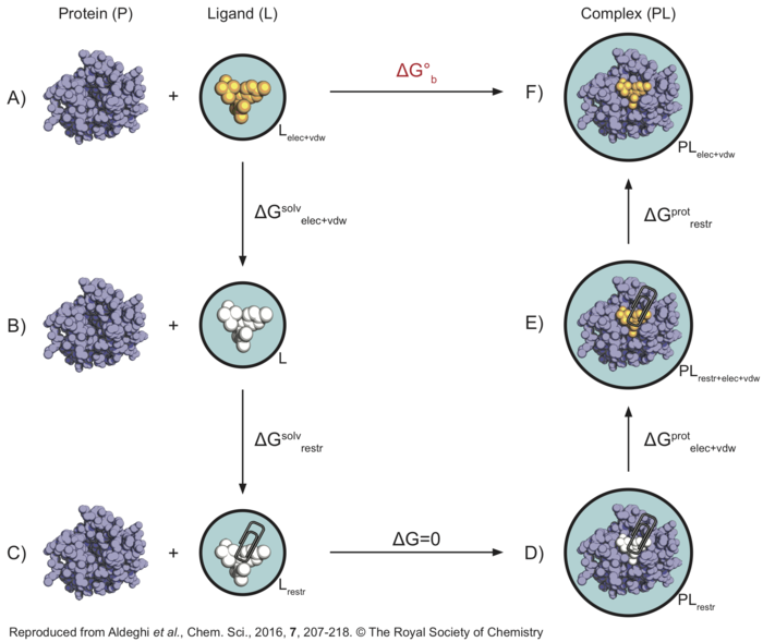
In this thermodynamic cycle, the systems we need to simulate are indicated by a black circle around them, the presence of restraints is indicated by a paperclip, a white ligand means it is not interacting with the environment (i.e. it is decoupled) and the light blue background is a reminder that explicit water is present. The right-hand side leg of the cycle involves simulations of the protein-ligand complex, whereas the left-hand side leg of the cycle involved simulations of the ligand in solution.
What we want to do is to go from to top-left corner of this cycle representing the physical unbound state (state A) to the top-right corner representing the physical bound state (state F), through a series of non-physical (or alchemical) intermediate states (like states B, C, D, and E). From the top-left corner of the cycle (state A), the first step is to decouple the ligand from solution (state B), in order to recover [math]\displaystyle{ \Delta G^{solv}_{elec+vdw} }[/math]. At this point the ligand is not interacting with the environment anymore, so that restraints are introduced in order to keep its position and orientation close to that of the bound pose. The free energy difference [math]\displaystyle{ \Delta G^{solv}_{restr} }[/math] between state B and C will be calculated analytically as described by Boresch et al.[2]. Also note that states C and D are effectively equivalent, since there are no interactions between the ligand (in vacuum) and protein (in solution) systems. Now the ligand's coulombic and vdW interactions are turned on again, and we can compute [math]\displaystyle{ \Delta G^{prot}_{elec+vdw} }[/math]. The ligand is however still restrained, which is not the physical bound state. Therefore, the restraints are finally removed through a series of simulations so that [math]\displaystyle{ \Delta G^{prot}_{restr} }[/math] can be calculated. Once all of the free energy differeces across the alchemical cycle have been calculated, the binding free energy ([math]\displaystyle{ \Delta G^{o}_{b} }[/math]) of the ligand can be recovered.
In this tutorial, we will always calculate the free energy for the decoupling of the ligand (going from top to bottom states of the cycle), since we find helpful to think of the ligand as being in the same state when at lambda=0 (coupled) versus lambda=1 (decoupled). However, this means that in order to sum all free energy terms correctly we will need to invert the sign of [math]\displaystyle{ \Delta G^{prot}_{elec+vdw+restr} }[/math].
Initial setup
In order to have everything ready to run the windows at different lambda values it is necessary to prepare all input files (.gro, .top and .mdp files); the typical Gromacs editconf/solvate/genion steps apply. Briefly, for this exercise the setup is as follows: dodecahedral box with minimum distance of 1.0 nm from the protein, Amber99SB-ILDN force field, TIP3P water model, GAFF parametrization for the ligand with AM1-BCC charges. More details about the parameters are in the .top and .mdp files provided, as well as in the original publication [1].
You can find the input files needed to complete this tutorial here: Input Files. As it is possible to see from the .mdp files, 20 windows will be used for the ligand in the solution leg of the cycle, and 30 for the protein-ligand complex leg of the cycle. A couple of things that is worth pointing out or reminding at this stage:
- Ligands with a net charge need to be treated with extra care as their decoupling will introduce artefacts (this is not the case for the ligand in this tutorial). There are also a couple of additional considerations for the setup of the simulation box, as this relates to the corrections one can then use (e.g. shape of the box, presence of counter ions). A discussion of these artefacts can be found >here< and the details on how to correct for them are in this paper by Rocklin et al.[3].
- It is important not to have atoms bearing a charge when the vdW interactions are decoupled (see this page for additional discussion). Thus, as you can see from the .mdp files, the charges are always decoupled before the vdW interactions.
- The run.sh scripts are there primarily to give an idea of how the whole set of simulations can be run. It is likely you will have to modify the gmx command in order to make it work with your installation. In particular for the complex, it can take several hours (or days) to run all simulations, so that you might not want to use up all of your cores. If you plan to use a cluster, you can still recycle this script if you wish to do so, but again you will probably need to adapt it.
- All .mdp files needed to run the calculations are provided. However, I also added a little mk_mdp.sh script (complex/MDP/mk_mdp.sh), which can help if you are preparing the files yourself, or if you do the calculations on your own system. Basically, it goes through the .mdp files it finds in the folder and replaces the string "$LAMBDA$" with numbers from 0 to N, where N is the number of states you have defined in any of the -lambda vectors. In this way, you can prepare a single mdp file with "init-lambda-state = $LAMBDA$" and then the script will generate all the .mdp files you need for the N states defined. For instance, if you prepare a "mymdpfile.mdp" with "coul-lambdas = 0.0 0.25 0.5 0.75 1.0", running "./mk_mdp.sh coul" will generate a folder called "MYMDPFILE" with 5 mdp files in it, one for each state defined in coul-lambdas with init-lambda-state from 0 to 4.
Ligand decoupling from complex
We will start taking care of the simulations of the complex, as they are more involved. This set of simulations comprises a total of 30 windows, and for each of them energy minimization, NVT and NPT equilibration, and production run (1 ns) are performed.
The set of restraints used is defined by 1 distance, 2 angles and 3 dihedrals harmonic potentials. These restraints have been defined by bonded terms between the ligand and the protein in the topology file (complex.top), using the [ intermolecular_interactions ] section with global indices. Note that this feature is present only in recent versions of Gromacs (5.1 and above); in older versions there is no such option and restraints can be applied only within one moleculetype. This complicates the setup substantially, as workarounds that involve a more extensive manipulation of the topology file are needed.
In the .mdp files we define 3 lambda vectors: bonded, coulomb, and vdw. In such a way we can use 30 identical .mdp files where we simply choose the state we are simulating with the init-lambda-state variable. As it is possible to see, we first apply the restraints, then we remove the coulombic, and finally the van der Waals interactions. Therefore, by decoupling the ligand, we are going from state F to D according to the thermodynamic cycle above.
We are now ready to run all the simulations and collect all the dhdl.xvg files needed for analysis. The run.sh script provided with the input files can be used to run the energy minimisation, NVT and NPT equilibrations, and production simulation for all lambda windows on your local machine, or it can be adapted to be used on some cluster. See Note 1 for Hamiltonian Replica Exchange.
Once all simulation are completed, it is possible to analyse the results with the alchemical_analysis.py python tool [4] available here. First, it helps to collect all dhdl.xvg files in a folder (e.g. using >this< simple script), then you can analyse all data with the following command:
alchemical_analysis.py -d 'directory' -p 'prefix' -t 300 -s 100 -u kcal -w -g
This will return the free energy estimate for going from state F to D ([math]\displaystyle{ \Delta G^{prot}_{elec+vdw+restr} }[/math]). To see all the options available, and their meaning, invoke the help by using the -h flag. If you prefer, you can also use the Gromacs tool gmx bar; however, I find alchemical-analysis to be more convenient as it already subsamples the data after calculating the statistical inefficiency, estimates the free energy with various methods (including BAR, MBAR and TI), and prints out results and some useful plots in a tidy format.
For this step of the calculations, with MBAR[5] I obtained:
[math]\displaystyle{ \Delta G^{prot}_{elec+vdw+restr} = 21.192 \pm 0.044 }[/math] kcal/mol
Here is a link to the output I obtained from the alchemical_analysis script: Results (Note 4). Note that this might not be exactly the number you will get (even if you use exactly the same input files, parameters and Gromacs version I used) but it should be close. In fact, running a total of free complex calculations, with MBAR I obtained a mean and standard deviation of [math]\displaystyle{ 21.181 \pm 0.093 }[/math] kcal/mol.
Ligand decoupling from solution
Now we need to obtain the free energy for the decoupling of the ligand from solution ([math]\displaystyle{ \Delta G^{solv}_{elec+vdw} }[/math]). This set of simulations involve a total of 20 windows. In this case we are only turning off coulombic and Lennard-Jones interactions, since the [math]\displaystyle{ \Delta G^{solv}_{restr} }[/math] can be calculated analytically as later shown.
The results can be obtained again in the same way as we did for the complex, and MBAR gave me:
[math]\displaystyle{ \Delta G^{solv}_{elec+vdw} = 7.739 \pm 0.021 }[/math] kcal/mol.
Restraints
Adding the restraints to the decoupled ligand (state B to C) can be taken into account analytically using Eq. 32 in Boresch et al.[2] (when using this specific set of restraints). The formula to use is the following, but it is suggested to first read the relevant paper to better understand where it comes from.
- [math]\displaystyle{ \displaystyle \Delta G^{solv}_{restr\_on} = RT \ln\Bigg[ \frac{8 \pi^{2}V^{0}}{r_{0}^{2} sin \theta_{A,0} sin \theta_{B,0}} \frac{(K_r K_{\theta_{A}} K_{\theta_{B}} K_{\phi_{A}} K_{\phi_{B}} K_{\phi_{C}})^{\frac{1}{2}}}{(2 \pi k T)^{3}}\Bigg] }[/math]
Where:
[math]\displaystyle{ R }[/math] is the ideal gas constant;
[math]\displaystyle{ T }[/math] is the temperature in Kelvin;
[math]\displaystyle{ V^{o} }[/math] is the volume corresponding to the one molar standard state (1660 Å[math]\displaystyle{ ^{3} }[/math]);
[math]\displaystyle{ r_0 }[/math] is the reference distance for the restraints;
[math]\displaystyle{ \theta_{A}, \theta_{B} }[/math] are the reference angles for the restraints;
[math]\displaystyle{ K_x }[/math] is the force constant for the distance ([math]\displaystyle{ r_0 }[/math]), two angles ([math]\displaystyle{ \theta_{A}, \theta_{B} }[/math]) and three dihedrals ([math]\displaystyle{ \phi_{A}, \phi_{B}, \phi_{C} }[/math]) restraints we applied.
You can use the restraints.py script provided to get the results of this equation (the values of the input variables, corresponding to the restraints defined in the topology, have already been set in this case, but you will need to change these if you use different equilibrium values or force constants). If you are using exactly the set of restraints provided with the input files, this should give 6.906 kcal/mol for turning the restraints on (-6.906 kcal/mol for turning them off, i.e. going from state C to B in the thermodynamic cycle). Note that the formula also contains the standard state correction.
Final Results
Now it is possible add all contributions to recover the binding free energy:
[math]\displaystyle{ \Delta G^{o}_{b} = - \Delta G^{prot}_{elec+vdw+restr} + \Delta G^{solv}_{elec+vdw} + \Delta G^{solv}_{restr\_on} }[/math]
Note that since we calculated the free energy difference for the decoupling (state F -> D) of the ligand from the complex, we now take its opposite. Based on the results mentioned above, I obtained:
[math]\displaystyle{ \Delta G^{o}_{b} = (-21.192 \pm 0.044) + (7.739 \pm 0.021) + 6.906 = -6.547 \pm 0.049 }[/math] kcal/mol
where the uncertainties have been compounded as the root sum square [math]\displaystyle{ \sqrt{\sigma_1^2+\sigma_2^2} }[/math], since they are for two independent free energy estimates.
In the specific case of this ligand there is also a symmetry correction to apply (Note 3)[6], because there is an alternative but equivalent binding pose in which the phenyl ring is flipped by 180 degrees. This secondary pose is not sampled during the short simulations of the protein-ligand complex due to the energy barrier to the ring flip. Furthermore, the use of restraints on the phenyl ring causes the secondary pose not to be energetically equivalent to the one sampled. This contribution due to symmetry amounts to [math]\displaystyle{ \Delta G_{sym} = -kT ln(2) = -0.413 }[/math] kcal/mol, so that the final result is:
[math]\displaystyle{ \Delta G^{o}_{b} = -6.960 \pm 0.049 }[/math] kcal/mol
It is possible to get a better idea of the precision of the protocol by running the whole calculation multiple times. With three repeats I obtained the following mean and standard deviation:
[math]\displaystyle{ \Delta G^{o}_{b} = -6.79 \pm 0.26 }[/math] kcal/mol.
Notes
(1) If you would like to use Hamiltonian Replica Exchange (HREX), you can simply add the -replex and -nex flags to mdrun when running the production simulations, after having already run all minimisations and equilibrations. The -multidir flag can be used to tell Gromacs where to find the .tpr file for all windows to be run in parallel.
mdrun -multidir lambda.*/PROD/ -s prod.tpr -deffnm prod -replex 1000 -nex 1000000
Here are the results I obtained by using HREX rather than separate simulations: HREX Results. If you compare the O_MBAR matrix obtained with HREX to the one obtained without it, you can see how using HREX resulted in better phase space overlap between states.
(2) Boyce et al.[1] applied a long range dispersion correction called EXP-LR to their final results. The EXP-LR method is described in Shirts et al., J. Phys. Chem. B, 2007.[7] What it does is basically correcting for the fact we are using a cutoff for the van der Waals interactions in a nonisotropic system. In the input files provided, however, the LJ-PME method was used for the treatment of the vdW interactions. Thus, the long-range part of the vdW interactions has already been accounted for directly during the simulations. In your calculations, you do not necessarily have to use LJ-PME, as it comes at additional computational cost. If you prefer, you can use the EXP-LR correction instead, or no correction at all. Taking the long-range LJ interactions into account properly will however make the results you obtain more reproducible, as they will not depend on the exact cutoff value chosen. In the old tutorial for Gromacs 4.6 you can find an explanation on how to obtain the EXP-LR correction. I would suggest to read the original paper first though.
(3) The symmetry correction is calculated as [math]\displaystyle{ -kT ln(\sigma) }[/math], where [math]\displaystyle{ \sigma }[/math] is the symmetry number, which here can apply to both the whole molecule and its substituents. The correction is needed if (a) the symmetric binding mode is not sampled during the simulations, and (b) the set of restraints used break the symmetry, causing the (in principle) equivalent conformation(s) to be energetically disfavoured. The paper by Mobley et al., J. Chem. Phys., 2006[6] has a more extensive discussion on the use of restraints and symmetry corrections in free energy calculations for who would like to delve deeper into the topic.
(4) You might notice that in the O_MBAR overlap matrix there are some suspicious vertical lines suggesting that some states overlap with almost all of the others (e.g. states 0, 3, 11, 16). This is due to the fact that the analysis script calculates long autocorrelation times for those windows, so that the effective number of uncorrelated samples found is less than the threshold set by the flag -i (50 by default). When this happens, the code then decides to consider all (correlated) samples provided. A possible consequence is that these states become highly populated and contain many more data points (10-100 times) as compared to the other states for which a smaller number of uncorrelated samples are considered. See this GitHub issue on the topic.
References
- ↑ 1.0 1.1 1.2 Boyce, S.E., Mobley, D.L., Rocklin, G.J., Graves, A.P., Dill, K.A., Shoichet, B.K. (2009) Predicting Ligand Binding Affinity with Alchemical Free Energy Methods in a Polar Model Binding Site. J. Mol. Biol. 394, 747–7636
- ↑ 2.0 2.1 Boresch, S., Tettinger, F., Leitgeb, M., and Karplus, M. (2003) Absolute binding free energies: A quantitative approach for their calculation. J. Phys. Chem. A 107, 9535–9551
- ↑ Rocklin, G.J., Mobley, D.A., Dill, K.A., Hünenberger, P.H. (2013) Calculating the binding free energies of charged species based on explicit-solvent simulations employing lattice-sum methods: An accurate correction scheme for electrostatic finite-size effects. J. Chem. Phys. 139, 184103
- ↑ Klimovich, P. V., Shirts, M. R., and Mobley, D. L. (2015) Guidelines for the Analysis of Free Energy Calculations. J. Comput. Aided. Mol. Des. 29(5), 397-411
- ↑ Shirts, M. R., and Chodera, J. D. (2008) Statistically optimal analysis of samples from multiple equilibrium states. J. Chem. Phys. 129, 124105
- ↑ 6.0 6.1 Mobley, D. L., Chodera, J. D., and Dill, K. A (2006) On the Use of Orientational Restraints and Symmetry Corrections in Alchemical Free Energy Calculations. J. Chem. Phys. 125, 084902
- ↑ Shirts, M. R., Mobley, D.L., Chodera, J. D., and Pande, V.S. (2007) Accurate and Efficient Corrections for Missing Dispersion Interactions in Molecular Simulations. J. Phys. Chem. B 111, 13052-13063